
# you can use Galaxy https://main.g2.bx.psu.edu/,
#Bedtools http://bedtools.readthedocs.org/en/latest/content/overview.html
#or Bioconductor package GenomicRanges #http://stuff.mit.edu/afs/athena/software/r_v2.14.1/lib/R/library/GenomicRanges/html/00Index.html
#python package HTSeq http://www-huber.embl.de/users/anders/HTSeq/doc/tour.html#tour
http://psaffrey.wordpress.com/2011/04/
Peter Saffrey's Weblog
Scientific computing and bioinformatics.
Overlapping Genomic Intervals Revisited
April 5, 2011
I’ve posted before on finding the right approach to overlapping genomic intervals. Broadly speaking, the problem is this: you have two sets of intervals, where each interval is (chromosome, start, end). You want to know where the intervals in the first set overlap the intervals in the second set.
For a while now, my go-to tool for this problem has been interval trees, which are a flexible and efficient data structure for inserting intervals from one set and making queries with the other. I have a cython implementation which is nice and fast.
Using an interval tree to find interval overlap has two stages:
However, many of my interval overlap applications are not like that. I have two sets of intervals and I want to find the overlaps between them once and then I’m done. I have to go through the expensive tree construction stage every time.
My alternative to this approach is to use a plane sweep algorithm. Conceptually, we build a list of the starts and ends of all the intervals from both sets, sorted in genomic order. Then we “sweep” from left to right recording when we enter and exit intervals from each set, and output when we’re in an interval from both. The problem is complicated slightly because with very large sets of intervals we don’t want to construct the whole list at the start, so I wanted to do the plane sweep dynamically, using pre-sorted lists of both sides and popping off items as I go.
After a bit of bashing, I got this working and the code is below: (I know this is verbose – it has quite a few comments)
This operates on two iterators of intervals,
A lot of the complicated logic happens in making the transition between chromosomes, particularly when there are gaps; both sets of intervals do not have intervals from the same chromosomes. This is where the algorithm relies on the chromosomes from both being in alphanumeric order, so that we can see if a chromosome is “before” another one. This works if we presort the intervals using (for example) the shell sort utility, and I have some wrapper functions to make this work with bed files:
So we sort the bed file into a temp file, and then
The plane sweep algorithm returns pairs of intervals, one from each set, which overlap. As well as the interval itself, it returns a 4th item which could be anything, so you could overlap objects (or whatever) to provide extra context in whatever application we’re writing. This is slightly different from the way the interval tree would be used, of which more later.
I ran some timing tests on this to compare it to my old faithful cython interval tree, using one tree for each chromosome. My test data was based on the mouse genome. On one side, I used the csp6i restriction enzyme (GTAC), a 4-base cutter we use in a lot of our 4C and Hi-C work; there are 5436400 in the mouse genome. On the other side, I generated random bed files of increasing numbers of 50bp reads – 10, 1000, 10000, 1000000, 2000000 and 5000000. I also did a 10 read example, to make sure the plane sweep algorithm could cope with gaps in the chromosome roster. I made sure both the interval tree and plane sweep methods identified the same intervals (the 10 read examples is missing for this plot, but I did make sure the overlaps were the same). I realise this test scheme is a little arbitrary but this is a typical use case for me, so it seemed like a good place to start.
Since it makes a difference whether you use the csp6i file as the tree or the query and as the “left” or “right” in the plane sweep, I tested it both ways. I did three tests of each. Below are the results, using the triplicate results to generate standard deviation error bars. Note that “git” stands for Genomic Interval Tree (one interval tree for each chromosome) and “PS” stands for Plane Sweep. Since the GIT method does not require the intervals to be sorted, every PS run includes the time it takes to sort the files first.

The plot headings refer to whether the csp6i file was on the left (“big-left” – which means it was used to build the interval trees) or the right (“big-right” – used as the queries). The plane sweep seems to perform much better than the interval trees for all the file sizes. The times are starting to ramp up at the 5,000,000 read level, but are still 10 times faster than the GIT method. I haven’t checked this, but it also ought to be much more memory efficient, since we’re not storing all the intervals in trees – we just visit each interval once to check its overlaps as we make the sweep.
As expected, the interval tree approach is much more efficient when we build a tree with the small number of intervals and make lots of queries on that tree. It makes a difference with the plane sweep too, since one side will have to make use of the more complicated caching machinery. I did a separate analysis to examine this:

To me, this is a good start, and I have already used the plane sweep approach to do some analysis work. I could probably speed it up even more by allowing the use of pre-sorted files. However, there are quite a few caveats:
I would also be interested to implement a multi-way plane sweep that overlaps several sets of intervals against a reference set. Maybe this would be quicker than building a tree for the reference set and comparing the others – something I still do very often.
-------------------------------------------------------------------
http://psaffrey.wordpress.com/2010/07/05/chromosome-interactions-heatmaps-and-matplotlib/
--------------------------------------------------------------
For a while now, my go-to tool for this problem has been interval trees, which are a flexible and efficient data structure for inserting intervals from one set and making queries with the other. I have a cython implementation which is nice and fast.
Using an interval tree to find interval overlap has two stages:
- Loading intervals into the tree to be queried.
- Querying those intervals.
However, many of my interval overlap applications are not like that. I have two sets of intervals and I want to find the overlaps between them once and then I’m done. I have to go through the expensive tree construction stage every time.
My alternative to this approach is to use a plane sweep algorithm. Conceptually, we build a list of the starts and ends of all the intervals from both sets, sorted in genomic order. Then we “sweep” from left to right recording when we enter and exit intervals from each set, and output when we’re in an interval from both. The problem is complicated slightly because with very large sets of intervals we don’t want to construct the whole list at the start, so I wanted to do the plane sweep dynamically, using pre-sorted lists of both sides and popping off items as I go.
After a bit of bashing, I got this working and the code is below: (I know this is verbose – it has quite a few comments)
1
2
3
4
5
6
7
8
9
10
11
12
13
14
15
16
17
18
19
20
21
22
23
24
25
26
27
28
29
30
31
32
33
34
35
36
37
38
39
40
41
42
43
44
45
46
47
48
49
50
51
52
53
54
55
56
57
58
59
60
61
62
63
64
65
66
67
68
69
70
71
72
73
74
75
| # uses a plane sweep to determine the overlaps between two sets of genomic intervals# they must come in as iterators# sorted, with the same chromosome orderdef overlapGeneratorPlaneSweep(left, right): # rightcache holds the points we've retrieved from the right set # that match the current left set chromosome, but we haven't finished filing yet rightcache = [] # nextcache holds points from right that from a later chromosome # to what we're currently looking at in left nextcache = [] lastchrom = None for linterval in left: lchrom, lstart, lend, lvalue = linterval # slight complex mechanics to handle a change in chromosome in left if lchrom != lastchrom: # still some left over in right # make sure there aren't any points leftover in right # from the last chromosome from left if rightcache != []: righti = rightcache[-1] while righti[0] < lchrom: righti = right.next() nextcache = [ righti ] rightcache = [] assert len(nextcache) <= 1 # the next cache is from a chromosome *before* the left chrom # suck up all the points from before left's chrom # - they will never overlap now if nextcache != [] and nextcache[0][0] < lchrom: righti = nextcache[0] while righti[0] < lchrom: righti = right.next() assert righti[0] >= lchrom nextcache = [ righti ] # if the point in nextcache matches the left chrom # nextcache is now current, so make it rightcach if nextcache != [] and nextcache[0][0] == lchrom: rightcache = nextcache[:] nextcache = [] assert rightcache == [] or rightcache[0][0] == lchrom # if the last point in the rightcache overlaps this left point, # there might be more points in the right that are relevant now while nextcache == [] and (rightcache == [] or rightcache[-1][1] <= lend): try: righti = right.next() except StopIteration: break if righti[0] == lchrom: rightcache.append(righti) elif righti[0] == lastchrom or (righti[0] == lchrom and righti[2] <= lstart): pass else: nextcache.append(righti) removecount = 0 # the bit where we actually check and report the overlaps for rinterval in rightcache: # we've gone past this one. Remove it if rinterval[2] <= lstart: removecount += 1 # we haven't reached this one yet. # We must have filed everything relevant from right. elif rinterval[1] >= lend: break else: # if we get here, this is an overlap. Yield it. yield((linterval, rinterval)) rightcache = rightcache[removecount:] lastchrom = lchrom |
left and right which must be sorted in the same chromosome order. We pop off an interval from left, and then pop off intervals from right, dropping those that are before the left interval and caching the others, until we go past the left interval. We report all the overlaps we found, and then pop the next left interval and continue.A lot of the complicated logic happens in making the transition between chromosomes, particularly when there are gaps; both sets of intervals do not have intervals from the same chromosomes. This is where the algorithm relies on the chromosomes from both being in alphanumeric order, so that we can see if a chromosome is “before” another one. This works if we presort the intervals using (for example) the shell sort utility, and I have some wrapper functions to make this work with bed files:
1
2
3
4
5
6
7
8
9
10
11
12
13
14
15
| import csvdef sortBedGenerator(bedfile): sortfile = bedfile + ".sort" cmd = "sort -k 1.4,1.5 -k 2,2n %s > %s" % (bedfile, sortfile) os.system(cmd) reader = csv.reader(open(sortfile), delimiter="\t") for row in reader: yield (row[0], int(row[1]), int(row[2]), 1) os.remove(sortfile)def overlapBedFilesPlaneSweep(leftbedfile, rightbedfile): leftgen = sortBedGenerator(leftbedfile) rightgen = sortBedGenerator(rightbedfile) return overlapGeneratorPlaneSweep(leftgen, rightgen) |
yield the sorted intervals one at a time.The plane sweep algorithm returns pairs of intervals, one from each set, which overlap. As well as the interval itself, it returns a 4th item which could be anything, so you could overlap objects (or whatever) to provide extra context in whatever application we’re writing. This is slightly different from the way the interval tree would be used, of which more later.
I ran some timing tests on this to compare it to my old faithful cython interval tree, using one tree for each chromosome. My test data was based on the mouse genome. On one side, I used the csp6i restriction enzyme (GTAC), a 4-base cutter we use in a lot of our 4C and Hi-C work; there are 5436400 in the mouse genome. On the other side, I generated random bed files of increasing numbers of 50bp reads – 10, 1000, 10000, 1000000, 2000000 and 5000000. I also did a 10 read example, to make sure the plane sweep algorithm could cope with gaps in the chromosome roster. I made sure both the interval tree and plane sweep methods identified the same intervals (the 10 read examples is missing for this plot, but I did make sure the overlaps were the same). I realise this test scheme is a little arbitrary but this is a typical use case for me, so it seemed like a good place to start.
Since it makes a difference whether you use the csp6i file as the tree or the query and as the “left” or “right” in the plane sweep, I tested it both ways. I did three tests of each. Below are the results, using the triplicate results to generate standard deviation error bars. Note that “git” stands for Genomic Interval Tree (one interval tree for each chromosome) and “PS” stands for Plane Sweep. Since the GIT method does not require the intervals to be sorted, every PS run includes the time it takes to sort the files first.

The plot headings refer to whether the csp6i file was on the left (“big-left” – which means it was used to build the interval trees) or the right (“big-right” – used as the queries). The plane sweep seems to perform much better than the interval trees for all the file sizes. The times are starting to ramp up at the 5,000,000 read level, but are still 10 times faster than the GIT method. I haven’t checked this, but it also ought to be much more memory efficient, since we’re not storing all the intervals in trees – we just visit each interval once to check its overlaps as we make the sweep.
As expected, the interval tree approach is much more efficient when we build a tree with the small number of intervals and make lots of queries on that tree. It makes a difference with the plane sweep too, since one side will have to make use of the more complicated caching machinery. I did a separate analysis to examine this:

To me, this is a good start, and I have already used the plane sweep approach to do some analysis work. I could probably speed it up even more by allowing the use of pre-sorted files. However, there are quite a few caveats:
- This is a very specific set of conditions. Before we could conclusively say the plane sweep approach was faster, there are lots of other conditions I would need to test:
- Different sizes of intervals.
- Many intervals within each group that overlap each other.
- Interval sizes that vary wildly within (and between) the groups.
- There is a lot of tuning possible on the structure of the interval trees that will affect performance.
- I’m not entirely comfortable with the reliance on coordinates in alphanumeric order here. It probably needs more error checking to make sure it reports if something goes wrong with that.
- As I mentioned, the way this should be used is different to the interval tree approach. With the csp6i sites, I usually want to look at a 4C read and say “is it near a csp6i site?” interval trees are a natural fit for this – I just query the tree, based on some tolerance for how near the site should be, and if I get any hits then I can act on those. To use the plane sweep approach, I need to change the layout of my code slightly to look for the presence of the read in the list of returned overlaps. I would also need to add an extra wrapper to generate intervals to take account of the tolerance I want to use. These are not insurmountable obstacles, but the plane sweep is not a drop-in replacement for the interval tree approach.
- Although comparing two sets of intervals is the basic use case, you always have to be wary of a one-size-fits-all approach. The plane sweep might be quicker for a pair of interval sets like this but, again with respect to the csp6i example, I might want to load the csp6i sites into a set of interval trees, and then query a list of 4C read-sets (lanes) against the tree. With only a few lanes of 4C, the plane sweep will probably still be quicker. How many lanes would I need before the interval tree approach becomes quicker again?
I would also be interested to implement a multi-way plane sweep that overlaps several sets of intervals against a reference set. Maybe this would be quicker than building a tree for the reference set and comparing the others – something I still do very often.
-------------------------------------------------------------------
http://psaffrey.wordpress.com/2010/07/05/chromosome-interactions-heatmaps-and-matplotlib/
Chromosome Interactions, Heatmaps and matplotlib
I’m currently working on some chromosome conformation data based on 3Cand related technologies. These tools allow you to look at the physical structure of the nucleus and determine how chromosomes are positioned in 3 dimensions, and where regions of one chromosome physically touch regions of another. These touching regions affect the regulation of genes in those regions.
The earlier iterations of these techniques are based on looking at interactions from a particular region or locus, to study the interaction with a specific set of genes. Later techniques allow a more flexible whole-genome approach. We are working with Hi-C data, which combines 3C/4C methods with paired-end sequencing, so that each end of the pair is at a different point on the genome.
After processing, this data is a neat list of interacting pairs, with each end as a chromosome coordinate. Our data produces between 2 and 10 million pairs. Most pairs are intra-chromosome (also called “cis” interactions) but around 5% are inter-chromosome (“trans” interactions).
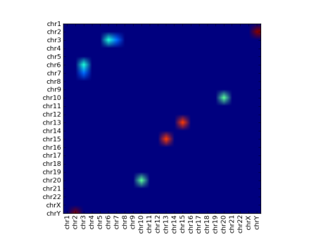
We now need a method to visualise this data. The prevalent method is theheatmap. The interaction points are grouped together into chromosomes, or regions of 100kb or 1mb (we could think of this as quantization). Interacting regions are marked out in a 2-dimensional matrix and then drawn as a heatmap.
For chromosome-chromosome heatmaps we might also normalise each spot based on the number of expected interactions. This is based on the length of the chromosomes – longer chromosomes should give more interactions on average. We also tend to remove cis-interactions – by reducing them to 0 – since otherwise they dominate and we can’t see the relative strengths of the trans-interactions.
Given the pairs of interactions, it’s easy enough to build the matrix that represents the interactions. Rendering this is matplotlib provides quite a few options. I’ve generated some sample data and showed a few options below, using the following code:
1
2
3
4
5
6
7
8
9
10
11
12
13
14
15
16
17
18
19
20
21
22
23
24
25
26
27
28
29
30
31
32
33
| import pylabchromnames = ['chr1', 'chr2', 'chr3', 'chr4', 'chr5', 'chr6', 'chr7', 'chr8', 'chr9', 'chr10', 'chr11', 'chr12', 'chr13', 'chr14', 'chr15', 'chr16', 'chr17', 'chr18', 'chr19', 'chr20', 'chr21', 'chr22', 'chrX', 'chrY']values = pylab.zeros((24, 24))values[2][6] = 3values[6][2] = 3values[23][1] = 13values[1][23] = 13values[5][2] = 5values[2][5] = 5values[12][14] = 11values[14][12] = 11values[19][9] = 6values[9][19] = 6f = pylab.Figure()#pylab.pcolor(values)#imagename = "pcolor.png"# pylab.imshow(values)# imagename = "imshow.png"pylab.matshow(values)imagename = "matshow.png"pylab.xticks(range(len(chromnames)), chromnames, rotation=90)pylab.yticks(range(len(chromnames)), chromnames)pylab.savefig(imagename) |
My first stab was to use imshow(), but this bleeds each coloured blob into the surroundings, which looks nice but makes it hard to read the individual blobs:
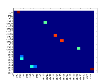
There is also a pcolor() function, but this plots from bottom to top (as you might expect) which is not ideal for what we want here. I’d have to turn the data and y axis labelling upside down, which is a little awkward:
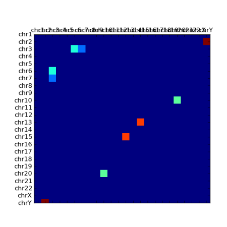
I finally plumped for matshow() (which stands for “matrix show”), which does things in the right order with solid blobs:
However it’s clearly not without its problems. The xtick labels have not rotated, so I had to do it manually, like this:
1
2
3
| im = pylab.matshow(values)for label in im.axes.xaxis.get_ticklabels(): label.set_rotation(90) |
You might also be able to see that the top and bottom rows are half-height – I had to correct this by adding dummy row labels here. I don’t know why this happens.
There are various other problems with the other plots too. I think it would be safe to say that matplotlib is a powerful tool but if you want plots in a particular way, it can take a lot of documentation bashing to get there. As always, I usually feel that the way I want it should be the standard and it should do that in the first place, but I can never tell how unreasonable I am being when I say this.
An open question here is whether heatmaps are actually the best way to visualise this data. I’m also working on a student project at the moment where we use a graph-based visualisation instead. My theory is that we can use a spring embedder algorithm to automatically lay out the graph of interactions between a pair of chromosomes and show their conformation. I think the usual wisdom here is that no visualisation is “right” – best to have several at your disposal to allow you to look at the data in a variety of different ways.
--------------------------------------------------------------
http://love-python.blogspot.com/
ReplyDeleteA python trick a day
see here for trees
ReplyDeletehere http://hackmap.blogspot.com/2008/11/python-interval-tree.html
and here http://code.google.com/p/bpbio/source/browse/trunk/interval_tree/interval_tree.py