I want to curate a public scRNAseq dataset from this paper Single-cell analyses reveal key immune cell subsets associated with response to PD-L1 blockade in triple-negative breast cancer
ffq
I first tried ffq, but it gave me errors.
ffq fetches metadata information from the following databases:
- GEO: Gene Expression Omnibus,
- SRA: Sequence Read Archive,
- EMBL-EBI: European Molecular BIology Laboratory’s European BIoinformatics Institute,
- DDBJ: DNA Data Bank of Japan,
- NIH Biosample: Biological source materials used in experimental assays,
- ENCODE: The Encyclopedia of DNA Elements.
(base) ➜  ~ ffq GSE169246
[2022-06-06 14:32:22,716]    INFO Parsing GEO GSE169246
[2022-06-06 14:32:24,418]    INFO Finding supplementary files for GEO GSE169246
[2022-06-06 14:32:28,001] WARNING There are 83 samples for GSE169246
[2022-06-06 14:32:28,001]    INFO Parsing GSM GSM5188367
[2022-06-06 14:32:33,047]    INFO Finding supplementary files for GSM GSM5188367
[2022-06-06 14:32:34,409]    INFO No supplementary files found for GSM5188367
[2022-06-06 14:32:39,659]    INFO Getting sample for GSM5188367
[2022-06-06 14:32:41,847] WARNING No sample found. Either the provided GSM accession is invalid or raw data was not provided for this record
get the metadata using GEOquery
other methods: pysradb https://github.com/saketkc/pysradb
I then tried GEOquery
library(GEOquery)
library(tidyverse)
library(here)
#getGEOSuppFiles(GEO ="GSE176021")
# one can also get the matrix by setting GSEMatrix to TRUE
meta<- getGEO(GEO= "GSE169246",GSEMatrix=FALSE)
The meta object’s gsms slot contains useful information
## metadata
meta@gsms$GSM5188440@header$characteristics_ch1#> [1] "tissue: blood" "disease state: TNBC patient"
#> [3] "group: Progression" "treatment: Chemo"## sample ID, I need it because the count matrix cell name is prefixed by it
meta@gsms$GSM5188440@header$title #> [1] "Prog_P008_b"## patient ID
meta@gsms$GSM5188440@header$source_name_ch1#> [1] "P008"meta@gsms is a list of lists. purrr::map() is a perfect tool to tidy it.
you can learn more purrr from https://jennybc.github.io/purrr-tutorial/
# each list entry is one sample
names(meta@gsms)#> [1] "GSM5188367" "GSM5188368" "GSM5188369" "GSM5188370" "GSM5188371"
#> [6] "GSM5188372" "GSM5188373" "GSM5188374" "GSM5188375" "GSM5188376"
#> [11] "GSM5188377" "GSM5188378" "GSM5188379" "GSM5188380" "GSM5188381"
#> [16] "GSM5188382" "GSM5188383" "GSM5188384" "GSM5188385" "GSM5188386"
#> [21] "GSM5188387" "GSM5188388" "GSM5188389" "GSM5188390" "GSM5188391"
#> [26] "GSM5188392" "GSM5188393" "GSM5188394" "GSM5188395" "GSM5188396"
#> [31] "GSM5188397" "GSM5188398" "GSM5188399" "GSM5188400" "GSM5188401"
#> [36] "GSM5188402" "GSM5188403" "GSM5188404" "GSM5188405" "GSM5188406"
#> [41] "GSM5188407" "GSM5188408" "GSM5188409" "GSM5188410" "GSM5188411"
#> [46] "GSM5188412" "GSM5188413" "GSM5188414" "GSM5188415" "GSM5188416"
#> [51] "GSM5188417" "GSM5188418" "GSM5188419" "GSM5188420" "GSM5188421"
#> [56] "GSM5188422" "GSM5188423" "GSM5188424" "GSM5188425" "GSM5188426"
#> [61] "GSM5188427" "GSM5188428" "GSM5188429" "GSM5188430" "GSM5188431"
#> [66] "GSM5188432" "GSM5188433" "GSM5188434" "GSM5188435" "GSM5188436"
#> [71] "GSM5188437" "GSM5188438" "GSM5188439" "GSM5188440" "GSM5188441"
#> [76] "GSM5188442" "GSM5188443" "GSM5188444" "GSM5188445" "GSM5585280"
#> [81] "GSM5585281" "GSM5585282" "GSM5585283"meta@gsms$GSM5188367@header#> $channel_count
#> [1] "1"
#>
#> $characteristics_ch1
#> [1] "tissue: blood" "disease state: TNBC patient"
#> [3] "group: Pre-treatment" "treatment: anti-PDL1+Chemo"
#>
#> $contact_address
#> [1] "Yiheyuan Road"
#>
#> $contact_city
#> [1] "Beijing"
#>
#> $contact_country
#> [1] "China"
#>
#> $contact_department
#> [1] "BIOPIC"
#>
#> $contact_email
#> [1] "zhangyuanyuanbio@pku.edu.cn"
#>
#> $contact_institute
#> [1] "Peking Univerisity"
#>
#> $contact_laboratory
#> [1] "Zemin Zhang's Lab"
#>
#> $contact_name
#> [1] "Yuanyuan,,Zhang"
#>
#> $contact_state
#> [1] "Beijing"
#>
#> $`contact_zip/postal_code`
#> [1] "100871"
#>
#> $data_processing
#> [1] "For 10X data, Cell Ranger 3.0.0 was used to quantify gene expression level, identify TCR sequences and quantify ATAC-seq peaks ."
#> [2] "Genome_build: GRCh38 for RNA expression,TCR data and ATAC peaks."
#>
#> $data_row_count
#> [1] "0"
#>
#> $description
#> [1] "10X Genomics platform"
#>
#> $extract_protocol_ch1
#> [1] "Peripheral blood mononuclear cells (PBMCs) were isolated with HISTOPAQUE-1077 (Sigma-Aldrich) solution. In brief, 3 ml fresh peripheral blood was collected at baseline, 4 weeks after treatment initiation and disease progression in EDTA anticoagulant tubes and subsequently layered onto HISTOPAQUE-1077. Tumor biopsy samples were first stored in RNAlater RNA stabilization reagent (QIAGEN) after collection and kept on ice to avoid RNA degradation. Samples were then collected in the RPMI-1640 medium (Gibco) with 10% FBS (Gibco), and enzymatically digested with gentle MACS Tumor Dissociation Kit (Miltenyi Biotec) for 60 min on a rotor at 37 °C according to the manufacturer’s protocol. The dissociated cells were next passed through a 40-µm cell-strainer (BD) in the RPMI-1640 medium (Invitrogen) with 10% FBS until uniform cell suspensions were obtained. Subsequently, the suspended cells were passed through cell strainers and centrifuged at 400 g for 10 min. Red blood cells were removed via the same procedure described above. After washing twice with 1x PBS (Invitrogen), the cell pellets were re-suspended in sorting buffer (PBS supplemented with 1% FBS)."
#> [2] "single cells were sorted into 1.5 ml tubes (Eppendorf) and counted manually under the microscope. The concentration of single cell suspensions was adjusted to 500-1200 cells/ul. Cells were loaded between 7,000 and 15,000 cells/chip position using the 10x Chromium Single cell 5’ Library, Gel Bead & Multiplex Kit and Chip Kit (10x Genomics, V3 barcoding chemistry) according to the manufacturer’s instructions. All the subsequent steps were performed following the standard manufacturer’s protocols. Purified libraries were analyzed by an Illumina Hiseq X Ten sequencer with 150-bp paired-end reads."
#> [3] "10x Chromium Single cell 5’ + VDJ Library, and 10x Chromium Single cell ATAC-seq Library"
#>
#> $geo_accession
#> [1] "GSM5188367"
#>
#> $instrument_model
#> [1] "HiSeq X Ten"
#>
#> $last_update_date
#> [1] "Sep 17 2021"
#>
#> $library_selection
#> [1] "cDNA"
#>
#> $library_source
#> [1] "transcriptomic"
#>
#> $library_strategy
#> [1] "RNA-Seq"
#>
#> $molecule_ch1
#> [1] "polyA RNA"
#>
#> $organism_ch1
#> [1] "Homo sapiens"
#>
#> $platform_id
#> [1] "GPL20795"
#>
#> $relation
#> [1] "BioSample: https://www.ncbi.nlm.nih.gov/biosample/SAMN18383051"
#>
#> $series_id
#> [1] "GSE169246"
#>
#> $source_name_ch1
#> [1] "P007"
#>
#> $status
#> [1] "Public on Sep 15 2021"
#>
#> $submission_date
#> [1] "Mar 19 2021"
#>
#> $supplementary_file_1
#> [1] "NONE"
#>
#> $taxid_ch1
#> [1] "9606"
#>
#> $title
#> [1] "Pre_P007_b"
#>
#> $treatment_protocol_ch1
#> [1] "Half of 22 TNBC patients were treated with paclitaxel monotherapy and the other half were treated with paclitaxel plus atezolizumab as first-line treatment"
#>
#> $type
#> [1] "SRA"# extract the metadata from the header
purrr::map(meta@gsms, ~.x@header$characteristics_ch1)[1:5]#> $GSM5188367
#> [1] "tissue: blood" "disease state: TNBC patient"
#> [3] "group: Pre-treatment" "treatment: anti-PDL1+Chemo"
#>
#> $GSM5188368
#> [1] "tissue: lymph_node" "disease state: TNBC patient"
#> [3] "group: Pre-treatment" "treatment: anti-PDL1+Chemo"
#>
#> $GSM5188369
#> [1] "tissue: blood" "disease state: TNBC patient"
#> [3] "group: Pre-treatment" "treatment: anti-PDL1+Chemo"
#>
#> $GSM5188370
#> [1] "tissue: lymph_node" "disease state: TNBC patient"
#> [3] "group: Pre-treatment" "treatment: anti-PDL1+Chemo"
#>
#> $GSM5188371
#> [1] "tissue: blood" "disease state: TNBC patient"
#> [3] "group: Pre-treatment" "treatment: anti-PDL1+Chemo"Also, have you used the awesome stack and unstack function in base R? There are so many good hidden functions.
# save it to a variable
meta1<- purrr::map(meta@gsms, ~.x@header$characteristics_ch1) %>%
        stack() %>%
        separate(values, into = c("condition", "value"), sep= ": ")%>%
        pivot_wider(names_from= condition, values_from = value) %>%
        janitor::clean_names()


meta2<- purrr::map(meta@gsms, ~.x@header$title) %>%
        stack() %>%
        dplyr::rename(sample_id = values)


meta3<- purrr::map(meta@gsms, ~.x@header$source_name_ch1) %>%
        stack() %>%
        dplyr::rename(patient_id = values)


head(meta1)#> # A tibble: 6 × 5
#> ind tissue disease_state group treatment
#> <fct> <chr> <chr> <chr> <chr>
#> 1 GSM5188367 blood TNBC patient Pre-treatment anti-PDL1+Chemo
#> 2 GSM5188368 lymph_node TNBC patient Pre-treatment anti-PDL1+Chemo
#> 3 GSM5188369 blood TNBC patient Pre-treatment anti-PDL1+Chemo
#> 4 GSM5188370 lymph_node TNBC patient Pre-treatment anti-PDL1+Chemo
#> 5 GSM5188371 blood TNBC patient Pre-treatment anti-PDL1+Chemo
#> 6 GSM5188372 blood TNBC patient Pre-treatment Chemohead(meta2)#> sample_id ind
#> 1 Pre_P007_b GSM5188367
#> 2 Pre_P007_t GSM5188368
#> 3 Pre_P012_b GSM5188369
#> 4 Pre_P012_t GSM5188370
#> 5 Pre_P014_b GSM5188371
#> 6 Pre_P023_b GSM5188372head(meta3)#> patient_id ind
#> 1 P007 GSM5188367
#> 2 P007 GSM5188368
#> 3 P012 GSM5188369
#> 4 P012 GSM5188370
#> 5 P014 GSM5188371
#> 6 P023 GSM5188372##merge all of them
meta<- left_join(meta1, meta2) %>%
left_join(meta3)
head(meta)#> # A tibble: 6 × 7
#> ind tissue disease_state group treatment sample_id patient_id
#> <fct> <chr> <chr> <chr> <chr> <chr> <chr>
#> 1 GSM5188367 blood TNBC patient Pre-treatm… anti-PDL… Pre_P007… P007
#> 2 GSM5188368 lymph_node TNBC patient Pre-treatm… anti-PDL… Pre_P007… P007
#> 3 GSM5188369 blood TNBC patient Pre-treatm… anti-PDL… Pre_P012… P012
#> 4 GSM5188370 lymph_node TNBC patient Pre-treatm… anti-PDL… Pre_P012… P012
#> 5 GSM5188371 blood TNBC patient Pre-treatm… anti-PDL… Pre_P014… P014
#> 6 GSM5188372 blood TNBC patient Pre-treatm… Chemo Pre_P023… P023## remove the scATACseq samples
meta<- meta %>%
filter(!str_detect(sample_id, "ATAC-seq"))Get the response data
Now, I will need to go to the publication and find the supplementary table which contains the response data. It looks like this:
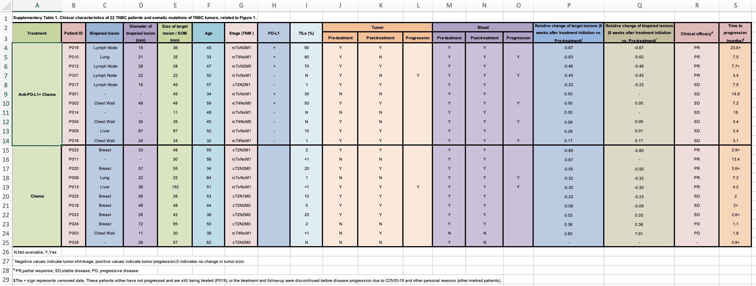 Everyone should read this https://datacarpentry.org/spreadsheet-ecology-lesson/02-common-mistakes/ and Data organization in spreadsheet
Using excel wisely is not a rocket science, but using it correctly can make bioinformatician’s life much easier.
clinical_data<- readxl::read_xlsx("~/Downloads/1-s2.0-S1535610821004992-mmc2.xlsx", skip = 1)

## there are many places need to be fixed
print(clinical_data, n = 40)
#> # A tibble: 27 × 19
#> Treatment `Patient ID` `Biopsied lesi…` `Diameter of b…` `Size of targe…`
#> <chr> <chr> <chr> <chr> <dbl>
#> 1 <NA> <NA> <NA> <NA> NA
#> 2 Anti-PD-L1+ … P019 Lymph Node 15 36
#> 3 <NA> P010 Lung 21 35
#> 4 <NA> P012 Lymph Node 28 28
#> 5 <NA> P007 Lymph Node 22 22
#> 6 <NA> P017 Lymph Node 16 45
#> 7 <NA> P001 - - 45
#> 8 <NA> P002 Chest Wall 48 48
#> 9 <NA> P014 - - 11
#> 10 <NA> P004 Chest Wall 35 35
#> 11 <NA> P005 Liver 87 97
#> 12 <NA> P016 Chest Wall 24 24
#> 13 Chemo P022 Breast 33 48
#> 14 <NA> P011 - - 30
#> 15 <NA> P020 Breast 37 55
#> 16 <NA> P008 Lung 22 22
#> 17 <NA> P013 Liver 36 152
#> 18 <NA> P025 Breast 26 26
#> 19 <NA> P018 Breast 48 48
#> 20 <NA> P023 Breast 26 42
#> 21 <NA> P024 Breast 72 95
#> 22 <NA> P003 Chest Wall 11 30
#> 23 <NA> P028 - 26 57
#> 24 N,Not availa… <NA> <NA> <NA> NA
#> 25 * Negative v… <NA> <NA> <NA> NA
#> 26 # PR,partial… <NA> <NA> <NA> NA
#> 27 $The + sign … <NA> <NA> <NA> NA
#> # … with 14 more variables: Age <dbl>, `Stage (TNM )` <chr>, `PD-L1` <chr>,
#> # `TILs (%)` <chr>, Tumor <chr>, ...11 <chr>, ...12 <chr>, Blood <chr>,
#> # ...14 <chr>, ...15 <chr>,
#> # `Relative change of target lesions (8 weeks after treatment initiation vs. Pre-treatment)*` <chr>,
#> # `Relative change of biopsied lesions (8 weeks after treatment initiation vs. Pre-treatment)*` <chr>,
#> # `Clinical efficacy#` <chr>, `Time to progression (months)$` <chr>## remove the first row and the last 4 rows, fill in the NAs for the Treatment
clinical_data<- clinical_data %>%
janitor::clean_names() %>%
slice(2:23) %>%
tidyr::fill(treatment) %>%
dplyr::select(!(tumor:x15)) yeah, and N for not available , and sometimes - means not available. let’s fix that.
clinical_data<- clinical_data %>%
        #trim off the white spaces. this will help the later step too
        mutate_all(~str_trim(.x, side ="both")) %>%
        mutate_at(vars(-pd_l1), ~str_replace(.x , "^-$", NA_character_)) %>%
        mutate_all( ~str_replace(.x , "^N$", NA_character_))
merge the two tables
meta<- meta %>%
        left_join(clinical_data) %>%
        arrange(patient_id, biopsied_lesion) %>%
        select(-biopsied_lesion)

print(meta, n = 20)#> # A tibble: 83 × 17
#> ind tissue disease_state group treatment sample_id patient_id
#> <fct> <chr> <chr> <chr> <chr> <chr> <chr>
#> 1 GSM5188381 blood TNBC patient Pre-treat… anti-PDL… Pre_P001… P001
#> 2 GSM5188414 blood TNBC patient Post-trea… anti-PDL… Post_P00… P001
#> 3 GSM5188376 blood TNBC patient Pre-treat… anti-PDL… Pre_P002… P002
#> 4 GSM5188377 chest_wall TNBC patient Pre-treat… anti-PDL… Pre_P002… P002
#> 5 GSM5188410 blood TNBC patient Post-trea… anti-PDL… Post_P00… P002
#> 6 GSM5188411 chest_wall TNBC patient Post-trea… anti-PDL… Post_P00… P002
#> 7 GSM5188437 blood TNBC patient Progressi… anti-PDL… Prog_P00… P002
#> 8 GSM5188401 chest_wall TNBC patient Post-trea… Chemo Post_P00… P003
#> 9 GSM5585280 blood TNBC patient Pre-treat… Anti-PD-… Pre_P004… P004
#> 10 GSM5585281 chest_wall TNBC patient Pre-treat… Anti-PD-… Pre_P004… P004
#> 11 GSM5585282 blood TNBC patient Post-trea… Anti-PD-… Post_P00… P004
#> 12 GSM5585283 blood TNBC patient Progressi… Anti-PD-… Prog_P00… P004
#> 13 GSM5188398 blood TNBC patient Pre-treat… anti-PDL… Pre_P005… P005
#> 14 GSM5188399 liver TNBC patient Pre-treat… anti-PDL… Pre_P005… P005
#> 15 GSM5188430 blood TNBC patient Post-trea… anti-PDL… Post_P00… P005
#> 16 GSM5188431 liver TNBC patient Post-trea… anti-PDL… Post_P00… P005
#> 17 GSM5188367 blood TNBC patient Pre-treat… anti-PDL… Pre_P007… P007
#> 18 GSM5188368 lymph_node TNBC patient Pre-treat… anti-PDL… Pre_P007… P007
#> 19 GSM5188402 blood TNBC patient Post-trea… anti-PDL… Post_P00… P007
#> 20 GSM5188433 blood TNBC patient Progressi… anti-PDL… Prog_P00… P007
#> # … with 63 more rows, and 10 more variables:
#> # diameter_of_biopsied_lesion_mm <chr>, size_of_target_lesion_som_mm <chr>,
#> # age <chr>, stage_tnm <chr>, pd_l1 <chr>, ti_ls_percent <chr>,
#> # relative_change_of_target_lesions_8_weeks_after_treatment_initiation_vs_pre_treatment <chr>,
#> # relative_change_of_biopsied_lesions_8_weeks_after_treatment_initiation_vs_pre_treatment <chr>,
#> # clinical_efficacy_number <chr>, time_to_progression_months <chr>That’s how much it takes to get the sample level metadata from a public dataset. It is hard to fully automate and one has to go to GEO and supplementary tables, and wrangle the data to a desired format. If you ask me, I will tell you this is the real-life bioinformatics.
Happy BioinFORMATics