Creative Commons License
This blog by Tommy Tang is licensed under a Creative Commons Attribution-ShareAlike 4.0 International License.

My github papge

Friday, July 25, 2014

run a local blast

I was checking the quality of a ChIP-seq fastq with fastqc, and the overrepresented sequence showed that the data contain Illumina Single End Adapter 1 contamination.

I have a file which contains all the possible illumina library sequences in fasta format (got from here), and I manually looked it and found that the single End Adapter 1 sequence did not match the report. I then was wondering  which sequence is the contamination. To do that, I have to do a local blast of  the overrepresented sequence "GATCGGAAGAGCTCGTATGCCGTCTTCTGCTTAGATCGGAAGAGCTCGTATGCC"
on the illumina library sequences.

Luckily, the ncbi_blast was installed on the HPC. One can follow the link here run local blast
first, use the formatdb command to convert the file to a database

$ module load ncbi_blast

# check what arguments are for the command
$ formatdb -

formatdb 2.2.26   arguments:

  -t  Title for database file [String]  Optional
  -i  Input file(s) for formatting [File In]  Optional
  -l  Logfile name: [File Out]  Optional
    default = formatdb.log
  -p  Type of file
         T - protein
         F - nucleotide [T/F]  Optional
    default = T
  -o  Parse options
         T - True: Parse SeqId and create indexes.
         F - False: Do not parse SeqId. Do not create indexes.
 [T/F]  Optional
    default = F
  -a  Input file is database in ASN.1 format (otherwise FASTA is expected)
         T - True,
         F - False.
 [T/F]  Optional
    default = F
  -b  ASN.1 database in binary mode
         T - binary,
         F - text mode.
 [T/F]  Optional
    default = F
  -e  Input is a Seq-entry [T/F]  Optional
    default = F
  -n  Base name for BLAST files [String]  Optional
  -v  Database volume size in millions of letters [Integer]  Optional
    default = 4000
  -s  Create indexes limited only to accessions - sparse [T/F]  Optional
    default = F
  -V  Verbose: check for non-unique string ids in the database [T/F]  Optional
    default = F
  -L  Create an alias file with this name
        use the gifile arg (below) if set to calculate db size
        use the BLAST db specified with -i (above) [File Out]  Optional
  -F  Gifile (file containing list of gi's) [File In]  Optional
  -B  Binary Gifile produced from the Gifile specified above [File Out]  Optional
  -T  Taxid file to set the taxonomy ids in ASN.1 deflines [File In]  Optional


$ formatdb -i adaptors_list.fa -o F -p F

several other files with names ended with nhr, nin and nsq are generated in the same directory.
then run blast:

# check argument for balstall
$ blastall -
blastall 2.2.26   arguments:

  -p  Program Name [String]
  -d  Database [String]
    default = nr
  -i  Query File [File In]
    default = stdin
  -e  Expectation value (E) [Real]
    default = 10.0
  -m  alignment view options:
0 = pairwise,
1 = query-anchored showing identities,
2 = query-anchored no identities,
3 = flat query-anchored, show identities,
4 = flat query-anchored, no identities,
5 = query-anchored no identities and blunt ends,
6 = flat query-anchored, no identities and blunt ends,
7 = XML Blast output,
8 = tabular,
9 tabular with comment lines
10 ASN, text
11 ASN, binary [Integer]
    default = 0
    range from 0 to 11
  -o  BLAST report Output File [File Out]  Optional
    default = stdout
  -F  Filter query sequence (DUST with blastn, SEG with others) [String]
    default = T
  -G  Cost to open a gap (-1 invokes default behavior) [Integer]
    default = -1
  -E  Cost to extend a gap (-1 invokes default behavior) [Integer]
    default = -1
  -X  X dropoff value for gapped alignment (in bits) (zero invokes default behavior)
      blastn 30, megablast 20, tblastx 0, all others 15 [Integer]
    default = 0
  -I  Show GI's in deflines [T/F]
    default = F
  -q  Penalty for a nucleotide mismatch (blastn only) [Integer]
    default = -3
  -r  Reward for a nucleotide match (blastn only) [Integer]
    default = 1
  -v  Number of database sequences to show one-line descriptions for (V) [Integer]
    default = 500
  -b  Number of database sequence to show alignments for (B) [Integer]
    default = 250
  -f  Threshold for extending hits, default if zero
      blastp 11, blastn 0, blastx 12, tblastn 13
      tblastx 13, megablast 0 [Real]
    default = 0
  -g  Perform gapped alignment (not available with tblastx) [T/F]
    default = T
  -Q  Query Genetic code to use [Integer]
    default = 1
  -D  DB Genetic code (for tblast[nx] only) [Integer]
    default = 1
  -a  Number of processors to use [Integer]
    default = 1
  -O  SeqAlign file [File Out]  Optional
  -J  Believe the query defline [T/F]
    default = F
  -M  Matrix [String]
    default = BLOSUM62
..........
..........

$ blastall -i overrepresented_sequence.fa -d adaptors_list.fa -p blastn -e 1e-6 

look at the result, I found that Adapter 2 is the contamination 
>Illumina_Single_End_Apapter_2
          Length = 34

 Score = 63.9 bits (32), Expect = 1e-14
 Identities = 32/32 (100%)
 Strand = Plus / Minus


Query: 1  gatcggaagagctcgtatgccgtcttctgctt 32
          ||||||||||||||||||||||||||||||||
Sbjct: 33 gatcggaagagctcgtatgccgtcttctgctt 2


I then feed Trimmomatic with this fasta file and removed the adaptor.


Tuesday, July 22, 2014

use python to change the header of a fasta file based on a dictionary in another file

I saw on SEQanwser, someone asked this question here, and I used python to resolve this problem.
I have not written in python for so long, I've been using R for a long time. This provide me a good practice opportunity.

The basic problem is to format some files, and I know it can be done by other tools like sed and awk ( see an awk solution below), but python just gives you much more flexibility in terms of what you can do and gives you more readability.
myfasta file

>comp1558_c0_seq1 len=204 path=[4976:0-203]
ATTGTACTTAATCTA.....
>comp8142_c0_seq1 len=222 path=[8835:0-221]
GTACAATCACGGCACATT......
>comp8570_c0_seq1 len=232 path=[3344:0-232]
GCATCGCTTATCGGTTTA......

annotation file:

comp1558_c0_seq1 repressor protein
comp8142_c0_seq1 aspartate aminotransferase
comp8357_c0_seq1 l-xylulose reductase
comp8387_c0_seq1 succinyl- synthetase alpha
comp8570_c0_seq1 fatty acid synthase beta subunit dehydratase

see the code below:


output:
>comp1558_c0_seq1 repressor protein
ATTGTACTTAATCTA.....
>comp8142_c0_seq1 aspartate aminotransferase
GTACAATCACGGCACATT......
>comp8570_c0_seq1 fatty acid synthase beta subunit dehydratase
GCATCGCTTATCGGTTTA......

if the dictionary file has only two records for each line, this awk should work:
http://stackoverflow.com/questions/11678939/replace-text-based-on-a-dictionary
NR == FNR {
  rep[$1] = $2
  next
} 

{
    for (key in rep) {
      gsub(key, rep[key])
    }
    print
}

Friday, July 4, 2014

get an idea of a gene expression value across samples by GEOquery

My next-door PI wanted to look at the TRIM29 expression levels in a series of tumor xenografts from a microarray data. I used GEOquery bioconductor package to get the log2 transformed values and plot a boxplot for him. see the code below. Also, I had a previous post on GEOquery http://crazyhottommy.blogspot.com/2013/12/geoquery-to-access-geo-datasets.html


after got the Expression set object, I looked the names of the object:
> names(pData(gset))
 [1] "title"                    "geo_accession"            "status"                   "submission_date"        
 [5] "last_update_date"         "type"                     "channel_count"            "source_name_ch1"        
 [9] "organism_ch1"             "characteristics_ch1"      "biomaterial_provider_ch1" "molecule_ch1"          
[13] "extract_protocol_ch1"     "label_ch1"                "label_protocol_ch1"       "taxid_ch1"              
[17] "source_name_ch2"          "organism_ch2"             "characteristics_ch2"      "biomaterial_provider_ch2"
[21] "molecule_ch2"             "extract_protocol_ch2"     "label_ch2"                "label_protocol_ch2"    
[25] "taxid_ch2"                "hyb_protocol"             "scan_protocol"            "description"            
[29] "data_processing"          "platform_id"              "contact_name"             "contact_email"          
[33] "contact_phone"            "contact_department"       "contact_institute"        "contact_address"        
[37] "contact_city"             "contact_state"            "contact_zip/postal_code"  "contact_country"        
[41] "supplementary_file"       "data_row_count"

then, only look at the meta data:
> pData(gset)[,c(1,2,28)]
                                 title geo_accession  description
GSM847887                  ML-5998-TG1     GSM847887    Xenograft
GSM847888              Baylor 2147 TG6     GSM847888    Xenograft
GSM847890             Baylor 2665A TG6     GSM847890    Xenograft
GSM847891              Baylor 3107 TG5     GSM847891    Xenograft
GSM847892              Baylor 3143 TG5     GSM847892    Xenograft
GSM847893              Baylor 3204 TG5     GSM847893    Xenograft
GSM847894              Baylor 3561 TG5     GSM847894    Xenograft
GSM847895              Baylor 3611 TG5     GSM847895    Xenograft
GSM847896             Baylor 3613A TG5     GSM847896    Xenograft
GSM847898              Baylor 3807 TG5     GSM847898    Xenograft
GSM847901              Baylor 3887 TG5     GSM847901    Xenograft
GSM847902              Baylor 3904 TG5     GSM847902    Xenograft
GSM847903              Baylor 3936 TG5     GSM847903    Xenograft
GSM847904              Baylor 3963 TG5     GSM847904    Xenograft
GSM847905              Baylor 4013 TG1     GSM847905    Xenograft
GSM847907              Baylor 4175 TG1     GSM847907    Xenograft
GSM847908              Baylor 4195 TG4     GSM847908    Xenograft
GSM847909              Baylor 4272 TG1     GSM847909    Xenograft
GSM847911              Baylor 4664 TG1     GSM847911    Xenograft
GSM847914              Baylor 4888 TG1     GSM847914    Xenograft
GSM847915              Baylor 4913 TG1     GSM847915    Xenograft
GSM847917                  ML-4189-TG2     GSM847917    Xenograft
GSM847919                  ML-5097-TG2     GSM847919    Xenograft
GSM847920                  ML-5156-TG2     GSM847920    Xenograft
GSM847921                  ML-5471-TG2     GSM847921    Xenograft
GSM847922 9830-000060B NEW PROTOCOL V5     GSM847922 Tumor sample
GSM847923            9830-000094B-244K     GSM847923 Tumor sample
GSM847924          9830-000424B-244Kv5     GSM847924 Tumor sample
GSM847925          9830-000517B-244Kv5     GSM847925 Tumor sample
GSM848100 9830-010118B NEW PROTOCOL V5     GSM848100 Tumor sample
GSM848101 9830-010130B NEW PROTOCOL V5     GSM848101 Tumor sample
GSM848102 9830-010214B NEW PROTOCOL V5     GSM848102 Tumor sample
GSM848103 9830-010255B NEW PROTOCOL V5     GSM848103 Tumor sample
GSM848104 9830-010384B NEW PROTOCOL V5     GSM848104 Tumor sample
GSM848105          9830-010461B-244Kv5     GSM848105 Tumor sample
GSM848106        9830-020018B-244K2008     GSM848106 Tumor sample
GSM848107          9830-020025B-244Kv5     GSM848107 Tumor sample
GSM848108          9830-020039B-244Kv5     GSM848108 Tumor sample
GSM848109        9830-020185B-244K2008     GSM848109 Tumor sample
GSM848110          9830-020310B-244Kv5     GSM848110 Tumor sample
GSM848111 9830-020340B NEW PROTOCOL V5     GSM848111 Tumor sample
GSM848112 9830-020416B NEW PROTOCOL V5     GSM848112 Tumor sample
GSM848113        9830-030267B-244K2008     GSM848113 Tumor sample
GSM848114          9830-030446B-244Kv5     GSM848114 Tumor sample
GSM848115        9830-030597B-244K2008     GSM848115 Tumor sample
GSM848116         UNC-000279B-244K2008     GSM848116 Tumor sample
GSM848117         UNC-010208B-244K2008     GSM848117 Tumor sample
GSM848118           UNC-010224B-244Kv5     GSM848118 Tumor sample
GSM848119           UNC-010304B-244Kv5     GSM848119 Tumor sample
GSM848120         UNC-010509B-244K2008     GSM848120 Tumor sample
GSM848121           UNC-020155B-244Kv5     GSM848121 Tumor sample
GSM848122             UNC-020320B-244K     GSM848122 Tumor sample
GSM848123         UNC-020578B-244k-DGE     GSM848123 Tumor sample
GSM848124         UNC-030065B-244K2008     GSM848124 Tumor sample
GSM848125         UNC-030183B-244K2008     GSM848125 Tumor sample
GSM848126         UNC-030370B-244K2008     GSM848126 Tumor sample
GSM848127         UNC-030528B-244K2008     GSM848127 Tumor sample
GSM848128         UNC-040011B-244K2008     GSM848128 Tumor sample
GSM848129           UNC-960028B-244Kv5     GSM848129 Tumor sample
GSM848130           WashU-15720-244Kv5     GSM848130 Tumor sample

there are 10 probes for TRIM29 gene:
> gpl_ann[gpl_ann$"Blast Gene Symbol"=="TRIM29",]
           ID    GB_ACC SPOT_ID Public id       Probe NAME Blast Gene ID Blast Refseq ID Blast Gene Symbol
35972   35972 NM_012101         NM_012101 NM_012101_2_2683         23650     NM_012101.3            TRIM29
39854   39854 NM_012101         NM_012101     A_23_P340123         23650     NM_012101.3            TRIM29
76447   76447 NM_012101         NM_012101     A_23_P340123         23650     NM_012101.3            TRIM29
94361   94361 NM_012101         NM_012101     A_23_P203267         23650     NM_012101.3            TRIM29
97602   97602 NM_012101         NM_012101 NM_012101_2_2608         23650     NM_012101.3            TRIM29
111151 111151 NM_012101         NM_012101 NM_012101_2_2683         23650     NM_012101.3            TRIM29
120477 120477 NM_012101         NM_012101     A_23_P203260         23650     NM_012101.3            TRIM29
132274 132274 NM_012101         NM_012101     A_23_P203260         23650     NM_012101.3            TRIM29
187541 187541 NM_012101         NM_012101 NM_012101_2_2608         23650     NM_012101.3            TRIM29
190531 190531 NM_012101         NM_012101     A_23_P203267         23650     NM_012101.3            TRIM29
               Blast Gene Description Blast Chromosome Map Location
35972  tripartite motif-containing 29                     11q22-q23
39854  tripartite motif-containing 29                     11q22-q23
76447  tripartite motif-containing 29                     11q22-q23
94361  tripartite motif-containing 29                     11q22-q23
97602  tripartite motif-containing 29                     11q22-q23
111151 tripartite motif-containing 29                     11q22-q23
120477 tripartite motif-containing 29                     11q22-q23
132274 tripartite motif-containing 29                     11q22-q23
187541 tripartite motif-containing 29                     11q22-q23
190531 tripartite motif-containing 29                     11q22-q23

the boxplot of the TRIM29 expression levels across different samples:


Thursday, June 26, 2014

quality control of your fastq file! my first post after I got my PhD!

I passed my defense on Tuesday, and now I am a PhD! what a long process, it took me six years. I've been enjoying the PhD experience though.

OK, let me go back to this post. things to remember:
1) You must quality control your fastq files first by fastqc. Trim the adapters and low quality bases by trimmomatic.
2) The fastq files dumped from the SRA GEO repository are usually the raw sequence, you need to quality control them.
3) google, google before you ask anyone else!

Let's start.
inspecting the first several reads of the fastq (this is a ChIP-seq data), I found the quality is coded as phred33

@SRR866627_nutlin_p53.1 HWI-ST571:161:D0YP4ACXX:3:1101:1437:2055 length=51
NCGAAAGACTGCTGGCCGACGTCGAGGTCCCGATTGTCGGCGTCGGCGGCA
+SRR866627_nutlin_p53.1 HWI-ST571:161:D0YP4ACXX:3:1101:1437:2055 length=51
#1:AABDDH<?CF<CFHH@D:??FAEE6?FHDAA=@CF@4@EBA88@;575
@SRR866627_nutlin_p53.2 HWI-ST571:161:D0YP4ACXX:3:1101:1423:2163 length=51
GAAATACTGTCTCTACTAAAAATACAAAAAGTAGCCAGGCGTCGTGGTGCA
+SRR866627_nutlin_p53.2 HWI-ST571:161:D0YP4ACXX:3:1101:1423:2163 length=51
B@CFFFFFHHHHGIJJJJIJJJIJJJJIJJIEGHIJJJJIJIIIHIE=FGC

To know different quality coding see here:
  SSSSSSSSSSSSSSSSSSSSSSSSSSSSSSSSSSSSSSSSS.....................................................
  ..........................XXXXXXXXXXXXXXXXXXXXXXXXXXXXXXXXXXXXXXXXXXXXXX......................
  ...............................IIIIIIIIIIIIIIIIIIIIIIIIIIIIIIIIIIIIIIIII......................
  .................................JJJJJJJJJJJJJJJJJJJJJJJJJJJJJJJJJJJJJJJ......................
  LLLLLLLLLLLLLLLLLLLLLLLLLLLLLLLLLLLLLLLLLL....................................................
  !"#$%&'()*+,-./0123456789:;<=>?@ABCDEFGHIJKLMNOPQRSTUVWXYZ[\]^_`abcdefghijklmnopqrstuvwxyz{|}~
  |                         |    |        |                              |                     |
 33                        59   64       73                            104                   126
  0........................26...31.......40                                
                           -5....0........9.............................40 
                                 0........9.............................40 
                                    3.....9.............................40 
  0.2......................26...31.........41                              

 S - Sanger        Phred+33,  raw reads typically (0, 40)
 X - Solexa        Solexa+64, raw reads typically (-5, 40)
 I - Illumina 1.3+ Phred+64,  raw reads typically (0, 40)
 J - Illumina 1.5+ Phred+64,  raw reads typically (3, 40)
     with 0=unused, 1=unused, 2=Read Segment Quality Control Indicator (bold) 
     (Note: See discussion above).
 L - Illumina 1.8+ Phred+33,  raw reads typically (0, 41)

then I used fastqc to check the quality:


the quality for each base is very good, but the perbase sequence content does not look good, and the adapters are not trimmed as indicated by the overrepresented sequences (highlighted part is part of the Truseq adapter index1).

Then I used Trimmomatic to trim the adapters and the low quality bases.
$ trimmomatic SE  in.fastq in_trimmed.fastq ILLUMINACLIP:Truseq_adaptor.fa:2:30:10 LEADING:3 TRAILING:3 SLIDINGWINDOW:4:15 MINLEN:36

the Truseq_adaptor.fa file contains the adapter sequences. see a post here.

$ cat Truseq_adaptor.fa
>TruSeq_Universal_Adapter
AATGATACGGCGACCACCGAGATCTACACTCTTTCCCTACACGACGCTCTTCCGATCT
>TruSeq_Adapter_Index_1
GATCGGAAGAGCACACGTCTGAACTCCAGTCACATCACGATCTCGTATGCCGTCTTCTGCTTG
>TruSeq_Adapter_Index_2
GATCGGAAGAGCACACGTCTGAACTCCAGTCACCGATGTATCTCGTATGCCGTCTTCTGCTTG
>TruSeq_Adapter_Index_3
GATCGGAAGAGCACACGTCTGAACTCCAGTCACTTAGGCATCTCGTATGCCGTCTTCTGCTTG
>TruSeq_Adapter_Index_4
GATCGGAAGAGCACACGTCTGAACTCCAGTCACTGACCAATCTCGTATGCCGTCTTCTGCTTG
>TruSeq_Adapter_Index_5
GATCGGAAGAGCACACGTCTGAACTCCAGTCACACAGTGATCTCGTATGCCGTCTTCTGCTTG
>TruSeq_Adapter_Index_6
GATCGGAAGAGCACACGTCTGAACTCCAGTCACGCCAATATCTCGTATGCCGTCTTCTGCTTG
>TruSeq_Adapter_Index_7
GATCGGAAGAGCACACGTCTGAACTCCAGTCACCAGATCATCTCGTATGCCGTCTTCTGCTTG
>TruSeq_Adapter_Index_8
GATCGGAAGAGCACACGTCTGAACTCCAGTCACACTTGAATCTCGTATGCCGTCTTCTGCTTG
>TruSeq_Adapter_Index_9
GATCGGAAGAGCACACGTCTGAACTCCAGTCACGATCAGATCTCGTATGCCGTCTTCTGCTTG
>TruSeq_Adapter_Index_10
GATCGGAAGAGCACACGTCTGAACTCCAGTCACTAGCTTATCTCGTATGCCGTCTTCTGCTTG
>TruSeq_Adapter_Index_11
GATCGGAAGAGCACACGTCTGAACTCCAGTCACGGCTACATCTCGTATGCCGTCTTCTGCTTG
>TruSeq_Adapter_Index_12
GATCGGAAGAGCACACGTCTGAACTCCAGTCACCTTGTAATCTCGTATGCCGTCTTCTGCTTG
after that, I checked the with fastqc again:


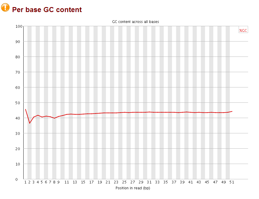
The perbase quality was improved and the per base GC content became more normal (should be 25% percent for each A,T,C,G base, it looks like the sequences are more A/T rich). More importantly, no overrepresent sequences were found anymore. Now the fastq file is ready for subsequent mapping by bowtie.

sometime ago, I quality controlled a RNA-seq data, and found found many wired things and asked on biostar.


Take home messages:
1)
"The weird per-base content is extremely normal and is typically referred to as the "random" hexamer effect, since things aren't actually amplified in a uniform manner. Most people will have this and it's nothing to worry about. BTW, don't let anyone talk you into trimming that off, it's the legitimate sequence."

2)
"Duplicates are expected in RNAseq. Firstly, your samples are probably full of rRNAs, even if you performed ribodepletion. Secondly, any highly expressed gene is going to have apparent PCR duplication due solely to it being highly expressed (there is a ceiling on the coverage you can get before running into this, it's pretty high with paired-end reads but not infinite)."

3)Several posts for whether the duplicates need to be removed or not.
https://www.biostars.org/p/55648/
https://www.biostars.org/p/66831/
https://www.biostars.org/p/14283/

Currently, I do not remove them. That's all for today!


Tuesday, June 17, 2014

& or && operator in R

I will defend next Tuesday. To relieve my anxiety a little bit, I decide to blog a little bit.

I am confused about the operator & and && in R, which one should I use?

It turns out:
"The shorter ones are vectorized, meaning they can return a vector, The longer form evaluates left to right examining only the first element of each vector"

an example would suffice to explain it.
> x<-c(1:10)
> x
 [1]  1  2  3  4  5  6  7  8  9 10
> x>8
 [1] FALSE FALSE FALSE FALSE FALSE FALSE FALSE FALSE  TRUE  TRUE
> logical1<- x>8
> logical2<- x<5
> logical1
 [1] FALSE FALSE FALSE FALSE FALSE FALSE FALSE FALSE  TRUE  TRUE
> logical2
 [1]  TRUE  TRUE  TRUE  TRUE FALSE FALSE FALSE FALSE FALSE FALSE
> logical1 | logical2
 [1]  TRUE  TRUE  TRUE  TRUE FALSE FALSE FALSE FALSE  TRUE  TRUE
> logical1 & logical2
 [1] FALSE FALSE FALSE FALSE FALSE FALSE FALSE FALSE FALSE FALSE
> logical1 && logical2
[1] FALSE
one can subset the vector by the logical vectors:
> x[logical1]
[1]  9 10
> x[logical2]
[1] 1 2 3 4


Tuesday, May 27, 2014

MACS for Dnase-seq data

It has been a long time since I posted last time. I will be defending at the end of next month. So, I am busy with my thesis writing. Anyway, I do want to keep a note here for using MACS to identify Dnase-seq peaks.

Although MACS was developed for ChIP-seq. It can also be used for Dnase-seq data. see a discussion here:
https://groups.google.com/forum/#!topic/macs-announcement/D1ZlzIJMBB8

several responses from the author of MACS Tao Liu:
Hi Zoello and Batool,
Any extension size is better than no extension at all. Even if there is no meaningful fragment size, signal pileup and data smoothing are still essential for peak detection algorithm. If you consider every tag only represents 0bp fragment, how can you decide where the enrichment is?
As for DNAseI hypersensitive studies, there are two scenarios. Using human ENCODE data as example, data from Duke university and University of Washington are generated by two different protocols. The key difference is the depth of digestion. DNA fragment captured is smaller in UW library comparing to Duke library due to different levels of digestion. In UW library, deep digestion and a gel cut for more smaller fragments can make sure the sequencing ends enriched at the boundaries of regions where the DNA is less accessible by the enzyme. These regions are more likely protected from DNaseI because of protein (TF, histone or other chromatin factors) binding in nuclei. So the following analysis can be considered similar to ChIP-seq where sonication tends to attack the boundaries of TF binding sites. In this case, tag extension towards 3' direction with hundreds of basepairs either from MACS prediction or an arbitrary setting, would work perfect. You can simply apply MACS on this kind of data. At the end, you will more likely predict where the DNA footprints are. However the sequencing tags from Duke are ends of bigger DNA fragments. So tag extension towards 3' direction may less likely reach where the real footprint is. In this case, the aim of the study should be to look for where the DNAseI hypersensitive sites are instead of to find footprints. My opinion is to extend every tag towards both 5' and 3' directions then pile them up, therefore at the end, the regions with more pileup would be more vulnerable to DNAseI digestion. If you want to use MACS for this purpose, you may need to manipulate the raw data then turn off model building in MACS.
That's my point of view. If anyone has difference opinion, please let us know."

"Of course you can use MACS2 on DNAse-seq data analysis. As for Hotspot, it uses a 250bps sliding window for calculation tag enrichment which is equivalent to a fixed 250bps extension in MACS2 setting.  As for number of peaks, it mainly depends on cutoff. Although DHS sites range from narrow to broad, there may still be an intrinsic fragment size in the library -- check your _model.pdf file from MACS2 or try Anshul's PhantomPeak tool. After all, this 'fragment size' is a factor for smoothing method, and an approximately correct smoothing is enough to improve peak detection. You may also try other methods without data smoothing, for example, SPP from Peter Park's lab or GPS from David Gifford's lab which can detect regions mainly based on forward and reverse reads balancing."


please read the related papers also:

Refined DNase-seq protocol and data analysis reveals intrinsic bias in transcription factor footprint identification 

http://www.nature.com/nmeth/journal/v11/n1/full/nmeth.2762.html

Current bioinformatic approaches to identify DNase I hypersensitive sites and genomic footprints from DNase-seq data
http://www.ncbi.nlm.nih.gov/pmc/articles/PMC3484326/

A Comparison of Peak Callers Used for DNase-Seq Data

http://www.plosone.org/article/info%3Adoi%2F10.1371%2Fjournal.pone.0096303

and a discussion on biostar 
https://www.biostars.org/p/70087/

Monday, April 14, 2014

order a matrix by a pre-defined group and then by the rowSums in R

I will lay down the R code below
#create a matrix

> mat<- matrix(sample.int(10, size=30, replace=T), ncol=3)
> mat
      [,1] [,2] [,3]
 [1,]    4    7    6
 [2,]    5    6    1
 [3,]    4    3    1
 [4,]    2    2    9
 [5,]    4    5    4
 [6,]    8    9    8
 [7,]    5    9    7
 [8,]    8    6    7
 [9,]    3    8    5
[10,]    4    3    6
# column bind the mat and the sum of the rows together 
> mat1<- cbind(mat, rowSums(mat))
> mat1
      [,1] [,2] [,3] [,4]
 [1,]    4    7    6   17
 [2,]    5    6    1   12
 [3,]    4    3    1    8
 [4,]    2    2    9   13
 [5,]    4    5    4   13
 [6,]    8    9    8   25
 [7,]    5    9    7   21
 [8,]    8    6    7   21
 [9,]    3    8    5   16
[10,]    4    3    6   13
# order the matrix by the rowSums(mat)
> mat[order(rowSums(mat)),]
      [,1] [,2] [,3]
 [1,]    4    3    1
 [2,]    5    6    1
 [3,]    2    2    9
 [4,]    4    5    4
 [5,]    4    3    6
 [6,]    3    8    5
 [7,]    4    7    6
 [8,]    5    9    7
 [9,]    8    6    7
[10,]    8    9    8
# compare with the order by looking at the last column
> mat1[order(rowSums(mat)),]
      [,1] [,2] [,3] [,4]
 [1,]    4    3    1    8
 [2,]    5    6    1   12
 [3,]    2    2    9   13
 [4,]    4    5    4   13
 [5,]    4    3    6   13
 [6,]    3    8    5   16
 [7,]    4    7    6   17
 [8,]    5    9    7   21
 [9,]    8    6    7   21
[10,]    8    9    8   25
# order the mat matrix in a decreasing order by adding a minus sign 
> mat[order(-rowSums(mat)),]
      [,1] [,2] [,3]
 [1,]    8    9    8
 [2,]    5    9    7
 [3,]    8    6    7
 [4,]    4    7    6
 [5,]    3    8    5
 [6,]    2    2    9
 [7,]    4    5    4
 [8,]    4    3    6
 [9,]    5    6    1
[10,]    4    3    1
# label the rows into different groups
> rownames(mat)<- c("f","a","d","c","b","d","e","a","f","f")
> mat
  [,1] [,2] [,3]
f    4    7    6
a    5    6    1
d    4    3    1
c    2    2    9
b    4    5    4
d    8    9    8
e    5    9    7
a    8    6    7
f    3    8    5
f    4    3    6
> rownames(mat1)<- c("f","a","d","c","b","d","e","a","f","f")
> mat1
  [,1] [,2] [,3] [,4]
f    4    7    6   17
a    5    6    1   12
d    4    3    1    8
c    2    2    9   13
b    4    5    4   13
d    8    9    8   25
e    5    9    7   21
a    8    6    7   21
f    3    8    5   16
f    4    3    6   13
> groups<- factor(rownames(mat))
> groups
 [1] f a d c b d e a f f
Levels: a b c d e f
# order the matrix by group first, and then within the subgroups, order by the rowSums
> mat1[order(groups,rowSums(mat)),] [,1] [,2] [,3] [,4] a 5 6 1 12 a 8 6 7 21 b 4 5 4 13 c 2 2 9 13 d 4 3 1 8 d 8 9 8 25 e 5 9 7 21 f 4 3 6 13 f 3 8 5 16 f 4 7 6 17
It is extremely useful when I want to order the matrix by a pre-defined way and then plot the heatmap with heatmap2 in gplots package.

Friday, April 11, 2014

rehead a bam file

I downloaded some ChIP-seq bam files from the UCSC genome browser http://hgdownload.cse.ucsc.edu/goldenPath/hg19/encodeDCC/wgEncodeHaibTfbs/

and I found some bam files headers  are without chrY information

samtools view -H  my.sorted.bam
@SQ SN:chr1 LN:249250621
@SQ SN:chr2 LN:243199373
@SQ SN:chr3 LN:198022430
@SQ SN:chr4 LN:191154276
@SQ SN:chr5 LN:180915260
@SQ SN:chr6 LN:171115067
@SQ SN:chr7 LN:159138663
@SQ SN:chr8 LN:146364022
@SQ SN:chr9 LN:141213431
@SQ SN:chr10 LN:135534747
@SQ SN:chr11 LN:135006516
@SQ SN:chr12 LN:133851895
@SQ SN:chr13 LN:115169878
@SQ SN:chr14 LN:107349540
@SQ SN:chr15 LN:102531392
@SQ SN:chr16 LN:90354753
@SQ SN:chr17 LN:81195210
@SQ SN:chr18 LN:78077248
@SQ SN:chr19 LN:59128983
@SQ SN:chr20 LN:63025520
@SQ SN:chr21 LN:48129895
@SQ SN:chr22 LN:51304566
@SQ SN:chrX LN:155270560
@SQ SN:chrM LN:16571

for some downstream analysis, I have to rehead this bam file:

samtools view -H my.bam | sed '24 a @SQ SN:chrY LN:59373566' | samtools reheader  -  my.bam > my.reheaded.bam

sed to append a line "@SQ SN:chrY LN:59373566" at  the 24th line
ctr+v+tab to insert a tab in the terminal.

Friday, April 4, 2014

liftover wig file

I was looking at a public ChIP-seq data set, but the author did not put the raw sequence data in the GEO database. Instead, they uploaded a wig file of the ChIP-seq signal file and it was mapped to human hg18 reference genome.

All the other data sets I am analyzing are mapped to hg19, so I have to liftover this wig file to hg19 also.

Solution: CrossMap! http://crossmap.sourceforge.net/

Convert Wiggle/BigWig format files

Wiggle (WIG) format is useful for displaying continuous data such as GC content and reads intensity of high-throughput sequencing data. BigWig is a self-indexed binary-format Wiggle file, and has the advantage of supporting random access. This means only regions that need to be displayed are retrieved by genome browser, and it dramatically reduces the time needed for data transferring (Kent et al., 2010). Input wiggle data can be in variableStep (for data with irregular intervals) or fixedStep (for data with regular intervals). Regardless of the input, the output will always in bedGraph format. bedGraph format is similar to wiggle format and can be converted into BigWig format using UCSC wigToBigWig tool. We export files in bedGraph because it is usually much smaller than file in wiggle format, and more importantly, CrossMap internally transforms wiggle into bedGraph to increase running speed.
If an input file is in BigWig format, the output is BigWig format if UCSC’s ‘wigToBigWig‘ executable can be found; otherwise, the output file will be in bedGraph format.
Typing command without any arguments will print help message:
$ python2.7 CrossMap.py  wig
Screen output:
Usage:
  CrossMap.py wig input_chain_file input_wig_file output_prefix

Description:
  "input_chain_file" can be regular or compressed (*.gz, *.Z, *.z, *.bz, *.bz2,
  *.bzip2) file, local file or URL (http://, https://, ftp://) pointing to remote
  file.  Both "variableStep" and "fixedStep" wiggle lines are supported. Wiggle
  format: http://genome.ucsc.edu/goldenPath/help/wiggle.html

Example:
  CrossMapy.py wig hg18ToHg19.over.chain.gz test.hg18.wig test.hg19

It is very easy to use, after install it following the instruction I did:
CrossMap.py wig hg18ToHg19.over.chain.gz my.wig my_hg19

it generates a bigwig file, a sorted bedgraph and a unsorted bedgraph file.

it took me 36mins to convert a 1.4Gb wig file on my desktop with 4Gb ram.