If you are doing research in biology, you will have to know how to use the Genome browsers:
UCSC genome browser, Ensemble, and the NCBI genome browser.
See a introduction here:
https://www.youtube.com/watch?v=vtJ6FvwCVTM&list=PLdmZ_rDf9sGScxV3bCR_QpDYaUpBY_CEA
I use UCSC genome browser a lot, mostly because of the rich annotation tracks. Sometimes, I go to Ensemble, it has a better view of sequences of exons and introns etc. I barely use the NCBI genome browser.
For Next Generation Sequencing analysis, you will be using some local genome browsers
IGV from Broad Institute http://www.broadinstitute.org/igv/
SeqMonk ,http://www.bioinformatics.babraham.ac.uk/projects/seqmonk/ it is excellent for some quantitation analysis of ChIP-seq, RNA-seq data.
MochiView, http://johnsonlab.ucsf.edu/mochi.html
it is really good for motif analysis besides the genome browsing function.
IGB http://bioviz.org/igb/, I have not used it personally
other browsers like Gbrowser
http://gmod.org/wiki/GBrowse
from the GMOD project is also an alternative.
http://gmod.org/wiki/Main_Page
Artemis from sanger Institute:
http://www.sanger.ac.uk/resources/software/artemis/
see a wiki link here: http://en.wikipedia.org/wiki/Genome_browser

This blog by Tommy Tang is licensed under a Creative Commons Attribution-ShareAlike 4.0 International License.
Thursday, May 30, 2013
Wednesday, May 29, 2013
Run APE plasmid editor in linux
I used to like APE on windows. I want to run it on linux (ubuntu 12.04 LTS) also.
A quick google search:
http://www.allandebono.org/ubuntu,ape/plasmid-editor/
I followed the instruction.
first download the APE for linux here http://biologylabs.utah.edu/jorgensen/wayned/ape/Download/
unzip it, you will find two folders, one for Linux, the other one for Mac_OS
copy the "APE linux" folder to your home directory: /home/tommy/APE_linux. I rename it as APE_linux, as linux "hates" the empty space.
cd /usr/bin
ls tclsh8.5
if you see it is there, you are fine. otherwise you have to install it:
sudo apt-get install tk8.5 tcl8.5
tclsh8.5 /home/tommy/APE_linux/AppMain.tcl

Thursday, May 23, 2013
Scaling variant detection pipelines for whole genome sequencing analysis from Blue collar bioinformatics
https://bcbio.wordpress.com/2013/05/22/scaling-variant-detection-pipelines-for-whole-genome-sequencing-analysis/?utm_source=feedlyBlue Collar Bioinformatics
Scaling variant detection pipelines for whole genome sequencing analysis
with 2 comments
Scaling for whole genome sequencing
Moving from exome to whole genome sequencing introduces a myriad of scaling and informatics challenges. In addition to the biological component of correctly identifying biological variation, it’s equally important to be able to handle the informatics complexities that come with scaling up to whole genomes.
At Harvard School of Public Health, we are processing an increasing number of whole genome samples and the goal of this post is to share experiences scaling the bcbio-nextgen pipeline to handle the associated increase in file sizes and computational requirements. We’ll provide an overview of the pipeline architecture in bcbio-nextgen and detail the four areas we found most useful to overcome processing bottlenecks:
- Support heterogeneous cluster creation to maximize resource usage.
- Increase parallelism by developing flexible methods to split and process by genomic regions.
- Avoid file IO and prefer streaming piped processing pipelines.
- Explore distributed file systems to better handle file IO.
This overview isn’t meant as a prescription, but rather as a description of experiences so far. The work is a collaboration between the HSPH Bioinformatics Core, the research computing team at Harvard FAS and Dell Research. We welcome suggestions and thoughts from others working on these problems.
Pipeline architecture
The bcbio-nextgen pipeline runs in parallel on single multicore machines or distributed on job scheduler managed clusters like LSF, SGE, and TORQUE. The IPython parallel framework manages the set up of parallel engines and handling communication between them. These abstractions allow the same pipeline to scale from a single processor to hundreds of node on a cluster.
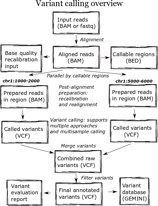
The high level diagram of the analysis pipeline shows the major steps in the process. For whole genome samples we start with large 100Gb+ files of reads in FASTQ or BAM format and perform alignment, post-alignment processing, variant calling and variant post processing. These steps involve numerous externally developed software tools with different processing and memory requirements.
Heterogeneous clusters
A major change in the pipeline was supporting creation of heterogeneous processing environments targeted for specific programs. This moves away from our previous architecture, which attempted to flatten processing and utilize single cores throughout. Due to algorithm restrictions, some software requires the entire set of reads for analysis. For instance,GATK’s base quality recalibrator uses the entire set of aligned reads to accurately calculate inputs for read recalibration. Other software operates more efficiently on entire files: the alignment step scales better by running using multiple cores on a single machine, since the IO penalty for splitting the input file is so severe.
To support this, bcbio-nextgen creates an appropriate type of cluster environment for each step:
- Multicore: Allocates groups of same machine processors, allowing analysis of individual samples with multiple cores. For example, this enables running bwa alignment with 16 cores on multiprocessor machines.
- Full usage of single cores: Maximize usage of single cores for processes that scale beyond the number of samples. For example, we run variant calling in parallel across subsets of the genome.
- Per sample single core usage: Some steps do not currently parallelize beyond the number of samples, so require a single core per sample.
IPython parallel provides the distributed framework for creating these processing setups, working on top of existing schedulers like LSF, SGE and TORQUE. It creates processing engines on distributed cores within the cluster, usingZeroMQ to communicate job information between machines.
Cluster schedulers allow this type of control over core usage, but an additional future step is to include memory and disk IO requirements as part of heterogeneous environment creation. Amazon Web Services allows selection of exact memory, disk and compute resources to match the computational step. Eucalyptus and OpenStack bring this control to local hardware and virtual machines.

Parallelism by genomic regions
While the initial alignment and preparation steps require analysis of a full set of reads due to IO and algorithm restrictions, subsequent steps can run with increased parallelism by splitting across genomic regions. Variant detection algorithms do require processing continuous blocks of reads together, allowing local realignment algorithms to correctly characterize closely spaced SNPs and indels. Previously, we’d split analyses by chromosome but this has the downside of tying analysis times to chromosome 1, the largest chromosome.
The pipeline now identifies chromosome blocks without callable reads. These blocks group by either genomic features like repetitive hard to align sequence or analysis requirements like defined target regions. Using the globally shared callable regions across samples, we fraction the genome into more uniform sections for processing. As a result we can work on smaller chunks of reads during time critical parts of the process: applying base recalibration, de-duplication, realignment and variant calling.

Streaming pipelines
A key bottleneck throughout the pipeline is disk usage. Steps requiring reading and writing large BAM or FASTQ files slow down dramatically once they overburden disk IO, distributed filesystem capabilities or ethernet connectivity between storage nodes. A practical solution to this problem is to avoid intermediate files and use unix pipes to stream results between processes.
We reworked our alignment step specifically to eliminate these issues. The previous attempt took a disk centric approach that allowed scaling out to multiple single cores in a cluster. We split an input FASTQ or BAM file into individual chunks of reads, and then aligned each of these chunks independently. Finally, we merged all the individual BAMs together to produce a final BAM file to pass on to the next step in the process. While nicely generalized, it did not scale when running multiple concurrent whole genomes.
The updated pipeline uses multicore support in samtools and aligners like bwa-mem and novoalign to pipe all steps as a stream: preparation of input reads, alignment, conversion to BAM and coordinate sorting of aligned reads. This results in improved scaling at the cost of only being able to increase single sample throughput to the maximum processors on a machine.
More generally, the entire process creates numerous temporary file intermediates that are a cause of scaling issues. Commonly used best-practice toolkits like Picard and GATK primarily require intermediate files. In contrast, tools in theMarth lab’s gkno pipeline handle streaming input and output making it possible to create alignment post-processing pipelines which minimize temporary file creation. As a general rule, supporting streaming algorithms amenable to piping can ameliorate file load issues associated with scaling up variant calling pipelines. This echos the focus on streaming algorithms Titus Brown advocates for dealing with large metagenomic datasets.
Distributed file systems
While all three of CPU, memory and disk speed limit individual steps during processing, the hardest variable to tweak is disk throughput. CPU and memory limitations have understandable solutions: buy faster CPUs and more memory. Improving disk access is not as easily solved, even with monetary resources, as it’s not clear what combination of disk and distributed filesystem will produce the best results for this type of pipeline.
We’ve experimented with NFS, GlusterFS and Lustre for handling disk access associated with high throughput variant calling. Each requires extensive tweaking and none has been unanimously better for all parts of the process. Much credit is due to John Morrissey and the research computing team at Harvard FAS for help performing incredible GlusterFS and network improvements as we worked through scaling issues, and Glen Otero, Will Cottay and Neil Klosterman at Dell for configuring an environment for NFS and Lustre testing. We can summarize what we’ve learned so far in two points:
- A key variable is the network connectivity between storage nodes. We’ve worked with the pipeline on networks ranging from 1 GigE to InfiniBand connectivity, and increased throughput delays scaling slowdowns.
- Different part of the processes stress different distributed file systems in complex ways. NFS provides the best speed compared to single machine processing until you hit scaling issues, then it slows down dramatically. Lustre and GlusterFS result in a reasonable performance hit for less disk intensive processing, but delay the dramatic slowdowns seen with NFS. However, when these systems reach their limits they hit a slowdown wall as bad or worse than NFS. One especially slow process identified on Gluster is SQLite indexing, although we need to do more investigation to identify specific underlying causes of the slowdown.
Other approaches we’re considering include utilizing high speed local temporary disk, reducing writes to long term distributed storage file systems. This introduces another set of challenges: avoiding stressing or filling up local disk when running multiple processes. We’ve also had good reports about using MooseFS but haven’t yet explored setting up and configuring another distributed file system. I’d love to hear experiences and suggestions from anyone with good or bad experiences using distributed file systems for this type of disk intensive high throughput sequencing analysis.
A final challenge associated with improving disk throughput is designing a pipeline that is not overly engineered to a specific system. We’d like to be able to take advantage of systems with large SSD attached temporary disk or wonderfully configured distributed file systems, while maintaining the ability scale on other systems. This is critical for building a community framework that multiple groups can use and contribute to.
Timing results
Providing detailed timing estimates for large, heterogeneous pipelines is difficult since they will be highly depending on the architecture and input files. Here we’ll present some concrete numbers that provide more insight into the conclusions presented above. These are more useful as a side by side comparison between approaches, rather than hard numbers to predict scaling on your own systems.
In partnership with Dell Solutions Center, we’ve been performing benchmarking of the pipeline on dedicated cluster hardware. The Dell system has 32 16-core machines connected with high speed InfiniBand to distributed NFS and Lustre file systems. We’re incredibly appreciative of Dell’s generosity in configuring, benchmarking and scaling out this system.
As a benchmark, we use 10x coverage whole genome human sequencing data from the Illumina platinum genomesproject. Detailed instructions on setting up and running the analysis are available as part of the bcbio-nextgen example pipeline documentation.
Below are wall-clock timing results, in total hours, for scaling from 1 to 30 samples on both Lustre and NFS fileystems:
| primary | 1 sample | 1 sample | 1 sample | 30 samples | 30 samples | |
|---|---|---|---|---|---|---|
| bottle | 16 cores | 96 cores | 96 cores | 480 cores | 480 cores | |
| neck | Lustre | Lustre | NFS | Lustre | NFS | |
| alignment | cpu/mem | 4.3h | 4.3h | 3.9h | 4.5h | 6.1h |
| align post-process | io | 3.7h | 1.0h | 0.9h | 7.0h | 20.7h |
| variant calling | cpu/mem | 2.9h | 0.5h | 0.5h | 3.0h | 1.8h |
| variant post-process | io | 1.0h | 1.0h | 0.6h | 4.0h | 1.5h |
| total | 11.9h | 6.8h | 5.9h | 18.5h | 30.1h |
Some interesting conclusions:
- Scaling single samples to additional cores (16 to 96) provides a 40% reduction in processing time due to increased parallelism during post-processing and variant calling.
- Lustre provides the best scale out from 1 to 30 samples, with 30 sample concurrent processing taking only 1.5x as along as a single sample.
- NFS provides slightly better performance than Lustre for single sample scaling.
- In contrast, NFS runs into scaling issues at 30 samples, proceeding 5.5 times slower during the IO intensive alignment post-processing step.
This is preliminary work as we continue to optimize code parallelism and work on cluster and distributed file system setup. We welcome feedback and thoughts to improve pipeline throughput and scaling recommendations.
Tuesday, May 21, 2013
Voom! Precision weights unlock linear model analysis tools for RNA-Seq read counts
http://www.rna-seqblog.com/data-analysis/expression-tools/voom-precision-weights-unlock-linear-model-analysis-tools-for-rna-seq-read-counts/
 This article revisits the idea of applying normal-based microarray-like statistical methods to RNA-seq read counts, with the idea that it is more important to model the mean-variance relationship correctly than it is to specify the exact probabilistic distribution of the counts. Log-counts per million are used as expression values. The voom method estimates the mean-variance relationship robustly and generates a precision weight for each individual normalized observation. The normalized log-counts per million and associated precision weights are then entered into the limma analysis pipeline, or indeed into any statistical pipeline for microarray data that is precision weight aware. This opens access for RNA-seq analysts to a large body of methodology developed for microarrays, allowing RNA-seq and microarray data to be analysed in closely comparable ways. The performance of voom and related limma-based pipelines is compared to that of edgeR, DESeq, baySeq, TSPM, PoissonSeq, and DSS. Simulation studies show that voom out-performs previous RNA-seq methods even when the data is generated according to the assumptions of the earlier methods. This is especially true when the sequence depths vary between RNA samples. Several data sets are also analysed to demonstrate how voom can handle heterogeneous data and complex experiments as well as facilitating pathway analysis and gene set testing methods.
Voom: variance modelling at the observation-level
In the past few years, RNA-seq has emerged as a revolutionary new technology for expression profiling. RNA-seq expression data consists of read counts, and many recent publications have argued therefore that RNA-seq data should be analysed by statistical methods designed specifically for counts. Yet all the statistical methods developed for RNA-seq counts rely on approximations of various kinds.
This article revisits the idea of applying normal-based microarray-like statistical methods to RNA-seq read counts, with the idea that it is more important to model the mean-variance relationship correctly than it is to specify the exact probabilistic distribution of the counts. Log-counts per million are used as expression values. The voom method estimates the mean-variance relationship robustly and generates a precision weight for each individual normalized observation. The normalized log-counts per million and associated precision weights are then entered into the limma analysis pipeline, or indeed into any statistical pipeline for microarray data that is precision weight aware. This opens access for RNA-seq analysts to a large body of methodology developed for microarrays, allowing RNA-seq and microarray data to be analysed in closely comparable ways. The performance of voom and related limma-based pipelines is compared to that of edgeR, DESeq, baySeq, TSPM, PoissonSeq, and DSS. Simulation studies show that voom out-performs previous RNA-seq methods even when the data is generated according to the assumptions of the earlier methods. This is especially true when the sequence depths vary between RNA samples. Several data sets are also analysed to demonstrate how voom can handle heterogeneous data and complex experiments as well as facilitating pathway analysis and gene set testing methods.Monday, May 20, 2013
what are phased and unphased genotypes?
I was reading about the format of the VCF file
http://www.1000genomes.org/node/101
" Genotype data are given for three samples, two of which are phased and the third unphased, with per sample genotype quality, depth and haplotype qualities (the latter only for the phased samples) given as well as the genotypes. The microsatellite calls are unphased."
what do phased and unphased mean?
a google search:
http://www.biostars.org/p/7846/
Phased data are ordered along one chromosome and so from these data you know the haplotype. Unphased data are simply the genotypes without regard to which one of the pair of chromosomes holds that allele.
Hi
actually (I think) phased or unphased status is not related to any measure of quality. For each individual, there are two chromosomes labelled (arbitrarily when you do not have genotypes of the parents) paternal and maternal. The names are self-explanatory.
For a haterozyguous genotype at a SNP position (which is called conditional on some quality score), you may know which allele is on the maternal chromosome and which one is on the paternal chromosome. The genotyped is "ordered". If you are able to assign, for a heterozyguous call (still conditional on the quality) at another SNP position which allele is on the paternal chromosome and which one is on the maternal, then you are able to phase these two SNPs - or more precisely, to phase the alleles at this SNPs. You then get an haplotype - or a suite of "ordered" SNPs.
In this context, having ordered 0/1 at SNP1 and 1/0 at SNP 2 is not the same as having 0/1 at SNP 1 and 1/0 at SNP 2.
First gives : 0 1 while second gives 0 0 __ __
1 0 1 1
Now, one could use some pre-estimated phase information on a panel population - typically different from the population where you call your alleles - to help calling an allele when the quality is low. This is what BEAGLECALL do, usually in a chip genotyping context.
As for the 1000 G data, having the phased data helps getting a better estimate of linkage disequilibrium. This also means that the format may differ so you need to take care when you take this as an input. But besides input format and more info about LD, the way you may use phased and unphased here are not really different.
Christian
PS : sorry if I went too far to the basics
Friday, May 17, 2013
Use tabix to extract subset of SAM, bed and VCF files
see here: http://davetang.org/muse/2013/02/22/using-tabix/
and here : http://www.biostars.org/p/43609/
and here: http://www.1000genomes.org/category/tabix
disclaimer: credits go to the original authors, refer to the links above for detailed
information.
-----------------------------------------------------------------------------------------------
and here : http://www.biostars.org/p/43609/
and here: http://www.1000genomes.org/category/tabix
disclaimer: credits go to the original authors, refer to the links above for detailed
information.
-----------------------------------------------------------------------------------------------
You can use tabix to extract subsets of the vcf files from the 1000genomes websites. Thanks to the fact that tabix uses a index file, you will be able to download only portions of the files, without having to download everything in local.
Example:
tabix -h ftp://ftp-trace.ncbi.nih.gov/1000genomes/ftp/release/20101123/interim_phase1_release/ALL.chr12.phase1.projectConsensus.genotypes.vcf.gz 1:10000,200000Using tabix
Tabix as described in the abstract of the paper:
Tabix is the first generic tool that indexes position sorted files in TAB-delimited formats such as GFF, BED, PSL, SAM and SQL export, and quickly retrieves features overlapping specified regions. Tabix features include few seek function calls per query, data compression with gzip compatibility and direct FTP/HTTP access. Tabix is implemented as a free command-line tool as well as a library in C, Java, Perl and Python. It is particularly useful for manually examining local genomic features on the command line and enables genome viewers to support huge data files and remote custom tracks over networks.
When I came across tabix a couple of years ago, I looked at the paper and also the man pageand while I felt it could be extremely useful, I didn't really appreciate the role it served. Now that I've seen what a colleague has achieved with it, I can see the light. Here I demonstrate with two simple examples some of the advantages of using tabix, namely speed and compression.
Testing tabix with SAM files
For the BAM file example, let's use one from The 1000 Genomes Project.
1
| wget ftp://ftp.1000genomes.ebi.ac.uk/vol1/ftp/data/NA18553/alignment/NA18553.chrom11.ILLUMINA.bwa.CHB.low_coverage.20120522.bam |
Now convert to SAM and index:
1
2
3
| samtools view -h NA18553.chrom11.ILLUMINA.bwa.CHB.low_coverage.20120522.bam > NA18553.chrom11.ILLUMINA.bwa.CHB.low_coverage.20120522.sambgzip NA18553.chrom11.ILLUMINA.bwa.CHB.low_coverage.20120522.samtabix -p sam NA18553.chrom11.ILLUMINA.bwa.CHB.low_coverage.20120522.sam.gz |
Of note is the file sizes:
1717942076 NA18553.chrom11.ILLUMINA.bwa.CHB.low_coverage.20120522.bam
1624632294 NA18553.chrom11.ILLUMINA.bwa.CHB.low_coverage.20120522.sam.gz
1624632294 NA18553.chrom11.ILLUMINA.bwa.CHB.low_coverage.20120522.sam.gz
bgzip compression of a SAM file is smaller than compressing to BAM; I can still use samtools with the bgzipped file though not as quick as processing a BAM file.
Now let's try some examples with tabix and samtools (samtools can also return reads within coordinates see this page) for returning reads mapped within genomic coordinates:
1
2
3
4
5
6
7
8
9
10
11
12
13
14
15
16
17
| tabix NA18553.chrom11.ILLUMINA.bwa.CHB.low_coverage.20120522.sam.gz 11:60000-70000SRR032291.13719341 163 11 60046 0 67M9S = 60358 346 TAAATACACTGAAGCTGCCAAAACAATCTATCGTTTTGCCTACGTACTTATCAACTTCCTCATAGCAACATGGGAG ?DEE?@BFDIHDGGHKHIHJHHF6H?<2HE?E>7:=3D7/CB=;.D?G@=)16.>@=+18+@(5@9########## X0:i:10 X1:i:0 XC:i:67 MD:Z:67 RG:Z:SRR032291 AM:i:0 NM:i:0 SM:i:0 MQ:i:0 XT:A:R BQ:Z:@@@@@@@@@@@@@@@@@@@@@@@@@@@@@@@@@@@@@@@@@@@@@@@@@@@@@@@@@@@@@@@@@@@@@@@@@@@@[rest of results snipped]time tabix NA18553.chrom11.ILLUMINA.bwa.CHB.low_coverage.20120522.sam.gz 11:60000-5000000 | wc 550668 11647956 203417916real 0m3.141suser 0m3.249ssys 0m1.524s#testing samtools using test.bed, which contains the coordinates 11 60000 5000000time samtools view -F 4 -L test.bed NA18553.chrom11.ILLUMINA.bwa.CHB.low_coverage.20120522.bam | wc 537327 11475465 200350980real 0m30.318suser 0m30.119ssys 0m1.800s |
Of note is the difference in the time taken to perform the calculations and the difference in the line numbers returned. The line difference is caused by tabix not taking into account the SAM/BAM flags, namely the unmapped flag. Though I don't show it here, I created a SAM file with one read with a SAM flag 4, which marks a read as being unmapped, but with chromosome coordinates and tabix still returned the read.
See here http://davetang.org/muse/2013/02/22/using-tabix/
Testing tabix with bed files
For the FANTOM5 project we have well over thousands of CAGE libraries. My aforementioned colleague prepared a bed file containing all the CAGE tags in all human samples. Despite having more than half a billion lines in this bed file, making a genomic inquiry took only seconds.
1
2
3
4
5
6
| time tabix hg19.ctss.bed.gz chr11:60000-5000000 | wc9577172 57463032 336697101real 0m6.276suser 0m7.997ssys 0m3.092s |
For the keen reader, have a look at the paper for tabix.
Subscribe to:
Comments (Atom)